Concept Drift vs Data Drift in Fine-Tuned Model Degradation

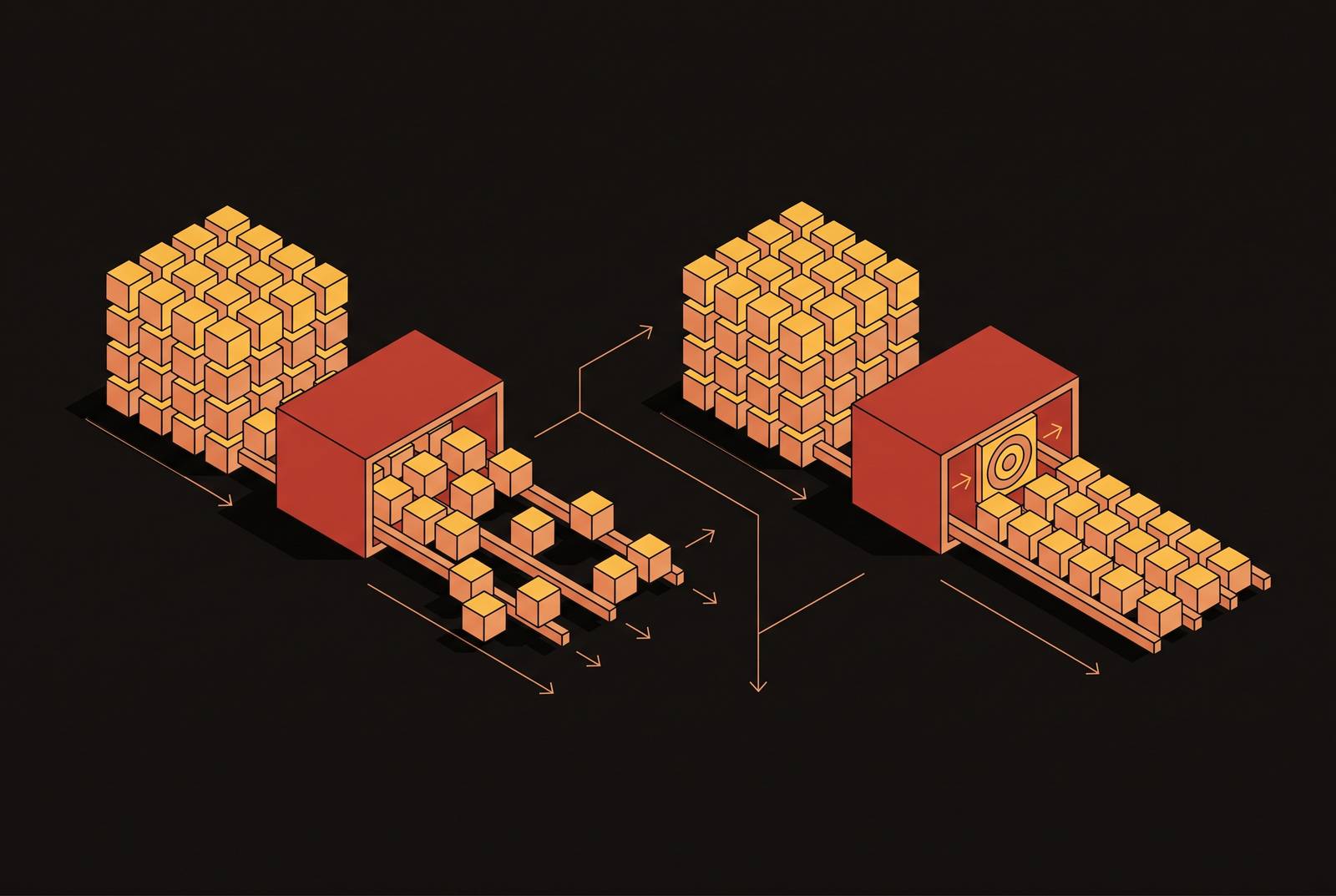
Fine-tuned model degradation requires a causal diagnosis. Data drift changes the inputs a model gets, while concept drift changes what the correct answer is for those inputs. This difference guides whether to update the training distribution or rebuild the learned relationship when maintaining the model. For CRM and RevOps systems, Quill’s emphasis on continuous data correction addresses the upstream reliability problem that makes both diagnoses harder.

Why fine-tuned models degrade: the two mechanisms that matter

“Model drift” names declining predictive performance without explaining its cause. Two mechanisms account for most degradation, and they invalidate different parts of a fine-tuned model’s training assumptions. Data drift changes the input distribution, written P(X), while the relationship between the inputs and the target stays the same. Concept drift changes that relationship, written P(y|X), so the same inputs now require a different output. A maintenance decision that treats these as interchangeable can target the wrong problem.

In CRM and RevOps systems, errors in records can damage the inputs to a model before that damage is visible in downstream predictions. Quill’s focus on continuous data correction bears on this upstream problem, which model-performance monitoring alone cannot diagnose. Yet neither drift mechanism necessarily interrupts operation or produces an obvious technical fault. Rabanser and colleagues describe machine learning systems as ones that “tend to fail silently,” with models continuing to return answers while accuracy erodes.

What data drift actually is and how it degrades a fine-tuned model

Data drift moves production inputs into parts of the feature space that the model saw little of during training. The pandemic retail example illustrates this mechanism. A demand forecasting model trained on how people shopped before the pandemic failed when they started buying more masks, sanitizers, and online purchases. In this example, the mapping from behavior to purchase remained unchanged, but the behaviors entering the model had moved. The model therefore faced a different mix of cases, including cases for which its learned boundary was weakly defined.

Statistically, P(X) changes while P(y|X) holds. This is covariate shift, which Lu and colleagues call “virtual drift” because the decision boundary does not move. The learned relationship remains valid in principle, but the training distribution no longer represents production well enough. A shift from desktop to mobile checkouts can change feature profiles without changing the prediction task. Seasonal demand, new customer segments, unfamiliar product names, and new regions can create the same mismatch.

Not every mismatch reflects genuine behavioral change. Upstream fields can switch units, imputation rules, or encoding schemes, changing what reaches the model without a corresponding change in the underlying business. These transformations can remain invisible to statistical drift detection, making continuous pipeline monitoring a separate requirement. Data-quality approaches, including Quill’s emphasis on correction within systems of record, address that upstream layer alongside model diagnostics.

Data drift has a useful detection advantage because comparing input distributions does not require outcome labels. Population Stability Index, KS tests, tests of categorical distributions, and embedding cosine drift can reveal changes before accuracy visibly falls. These signals establish that inputs have moved while leaving the effect on predictions undetermined. Because the target relationship remains valid, remediation centers on restoring alignment between training and production while preserving the prediction task.

What concept drift actually is and why it is harder to fix

Concept drift changes P(y|X), making the correct answer different for an otherwise familiar input. Fraud detection provides the canonical example. Once a model learns a fraud pattern, fraudsters can shift toward transactions that resemble approved ones. The same features then carry a different risk, even if the input distribution looks familiar. The model’s decision boundary is now out of date, beyond any change in which inputs the model sees.

This makes concept drift structurally harder and more expensive to fix than data drift. More examples of current inputs are insufficient if their labels still express the old relationship. New labels must capture outcomes under the changed conditions, but those outcomes may not be available when predictions are made. A recession can change default risk at the same income, and a policy change can redefine which transactions count as compliant. In both cases, old labels can actively teach the wrong answer.

Lu’s review distinguishes four forms of this change. Sudden drift changes the relationship at once, as when a regulation takes effect. Gradual drift allows old and new relationships to alternate until the new one dominates. With incremental drift, the relationship changes a little at a time without stopping, while recurring drift brings back an earlier relationship. The distinction matters because a temporary return to a known relationship presents a different maintenance problem from a structural break that makes historical training data unsuitable.

TU Delft’s McUDI paper (2024) highlights prior research showing that AIOps failure-prediction models do not generalize well to future data under continuous concept drift from workloads and hardware/software upgrades. It also notes that labeling costs can make periodic retraining infeasible. The paper reports monetary losses from AIOps service interruptions caused by model-quality degradation in the range of $300,000 to $400,000. This illustrates the combined burden of degraded predictions and expensive corrective evidence. Where a structural break has occurred, retraining on past data cannot restore a relationship that no longer exists.

How the two drifts interact and why they often arrive together

Co-occurrence is a normal production condition. A single economic change can alter both the population entering a model and the outcomes associated with that population. A recession, for example, can change who applies for loans while also changing who defaults at the same income level. The first change affects P(X), while the second affects P(y|X). Detecting either one therefore does not establish that it alone caused an accuracy decline.

An input-distribution test can flag a change even when performance stays the same because the model still handles the new inputs well. Inputs can also stay the same while the relationship changes and accuracy falls. When input shift and degraded performance appear together, data drift is plausible, but concept drift remains possible. Diagnosis requires evidence about both the inputs and the correctness of the outputs.

Retrieval-augmented systems add another layer to that reasoning. The same prompt can retrieve different supporting documents, changing the effective P(answer | prompt) even though the user’s wording remains stable. Viewed at the prompt level, this retrieval drift behaves more like a relationship shift than a simple change in prompt distribution. It is nevertheless a pipeline-level change, which shows why the observation boundary matters. Monitoring only the user’s prompt can miss a material change in what determines the answer.

How to tell which drift type is occurring in a production system

The practical sequence is to check inputs, check output quality, and then assess whether the two move together or independently. Population Stability Index compares bucketed reference and production distributions, with a value above 0.2 signaling significant drift on a feature. KS tests serve continuous features, but their p-value thresholds need calibration to avoid alert fatigue at scale. Chi-square tests serve categorical features. For high-dimensional inputs, cosine drift compares embedding centroids, while Maximum Mean Discrepancy provides a non-parametric two-sample test on embeddings without binning.

The second measurement establishes whether predictive performance has actually deteriorated. Classical models can be assessed through accuracy, precision, recall, F1, calibration error, and Brier score. LLM and agent systems instead require measures such as faithfulness, groundedness, answer relevancy, refusal rates, and tool-call accuracy from production traces. When outcomes come in late, Confidence-Based Performance Estimation or Distribution-based Label-free Estimation can estimate how well the model is doing before labels are available. Those estimates help bridge label lag, but they do not remove the need to understand whether the target relationship has changed.

The joint reading produces four diagnostic cases. When inputs shift but accuracy stays the same, it suggests a harmless covariate shift that the model can handle, so the model should be monitored and immediate retraining can wait. Input shift with degraded accuracy makes data drift a plausible cause and supports updating the training distribution, while leaving concept drift as an unresolved possibility. Stable inputs with degraded accuracy provide a strong signal of concept drift and a need for new labels. Evidence that both the input distribution and conditional relationship have shifted indicates co-occurrence, requiring the concept drift component to be addressed first.

Model relevance can make input monitoring more useful. TU Delft’s McUDI paper uses the trained model’s feature-importance ranking to choose the features that matter most and runs KS tests on them. This gives a sign of degradation without needing labels and gives more weight to changes in the distributions of the features that matter most. For LLM systems, the diagnostic view also needs prompt structure, including length, language mix, and intent class. Retrieval embedding distances and per-trace output-quality evaluations then reveal changes that prompt-distribution monitoring alone would miss.

What the right fix looks like once you have a diagnosis

The remediation asymmetry is decisive. Data drift permits reuse of the model’s learned relationship, whereas concept drift requires learning the changed relationship. For data drift, teams can retrain on a representative production dataset, reweight samples toward recent data, or repair the upstream pipeline when the shift is a data-quality artifact. For LLM systems, prompt feature engineering or retrieval-index reweighting may substitute for full retraining.

Concept drift requires labels collected under the new relationship. In a sudden structural break, past data may need to be discarded or heavily downweighted because it describes conditions that no longer apply. Recurring drift may instead favor an ensemble or switching strategy that selects the appropriate learned relationship for the period. TU Delft’s McUDI paper offers a cost-reduction approach by shifting retraining from a fixed schedule to degradation-triggered retraining. When both drifts occur, restoring the correct relationship takes priority over updating the input distribution.

This distinction has concrete consequences for CRM and RevOps AI. Contact records go out of date as people change jobs, companies restructure, and contact details grow stale. Job titles, direct-dial phone numbers, business emails, and company firmographics are also inputs on which GTM AI depends. At the same time, the relationship between those attributes and conversion, response, or churn changes with markets and buyer preferences. A familiar firmographic profile can therefore become less predictive even after its fields have been corrected.

Corrective training data can compound the problem if it contains mislabeled outcomes, duplicate records, or corrupted features. In that setting, Quill’s data-correction premise is relevant to the reliability of the retraining inputs. Batch cleanup fixes record problems that have built up, while continuous correction fixes them between a business change and the next cleanup cycle. When change happens monthly and cleanup happens quarterly, agents inherit a system of record that is structurally behind. Defaulting to “retrain on more recent data” misses this distinction and can preserve obsolete labels in an apparently current dataset.

Why alerting alone is not a maintenance strategy for drift

A correct diagnosis only matters if it leads to a timely response. Downstream accuracy alerts arrive after a model has already returned unreliable outputs for some period. Lost transactions, misfired workflows, and corrupted dashboards can accumulate during that interval. Concept drift lengthens the exposure because confirmed outcomes may lag predictions by days, weeks, or more. Waiting for a label-dependent alarm therefore leaves a gap between the changed relationship and the system’s response.

Continuous input monitoring reduces that gap for data drift, while output-quality monitoring on every production trace or a sampled stream addresses degradation as early as the available evidence allows. The signals must be read together so that harmless changes in the inputs do not lead to retraining the model needlessly. They must also stay linked to upstream data-quality monitoring, which can show changes that model-level statistics miss. In systems of record, audits every quarter cannot keep up with CRM data that changes all the time. Monitoring needs a path from detection through notification to correction.

Quill expresses that operational premise through agents intended to find anomalies, propose corrections, and apply fixes autonomously. That role complements statistical monitoring and model retraining. The broader architectural requirement follows from the two drift mechanisms themselves. Changes in inputs need to be fixed early, while changes in relationships call for new evidence and a change in what the model learns. An agentic system can connect those diagnoses to action, whereas alerting alone leaves the maintenance loop open.